Geospatial Search Introduction
A user in Times Square opens a food delivery app and searches for pizza places within 2km. The database holds 10 million restaurant locations. A traditional B-tree index on latitude finds 50,000 restaurants in the right latitude band. But restaurants at the same latitude can be 20km apart in longitude. The app must calculate distance for all 50,000 candidates.
Traditional database indexes organize data along a single dimension. Proximity searches span two dimensions simultaneously. This mismatch forces full table scans on the second dimension.
Why Standard Indexes Fail
B-trees excel at finding exact matches and range queries on single dimensions. They efficiently find all users named "John" or orders between two dates. But proximity searches span two dimensions: latitude and longitude.
A B-tree can index latitude efficiently. But filtering by longitude afterward still requires scanning thousands of records. For 10 million restaurants, a naive proximity search calculates distance for every record:
distance = sqrt((lat2 - lat1)² + (lng2 - lng1)²)
This distance calculation repeated millions of times creates unacceptable latency. Spatial indexing solves this by organizing locations geographically, cutting the candidate set from 10 million comparisons to, illustratively, on the order of hundreds.
Tree-Based Indexing
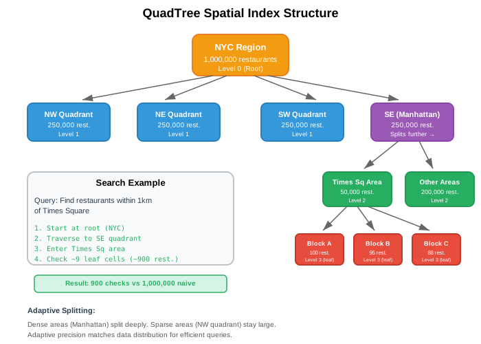
QuadTrees divide space recursively into four quadrants. Each node represents a geographic region. When a region contains too many points, it splits into four children.
This adapts to data density. Manhattan with 10,000 restaurants per square kilometer splits deeply. Rural Wyoming with one restaurant per 100 square kilometers stays as large cells.
Search process:
A user at Times Square searches for restaurants within 1km. The QuadTree starts at the root covering all of NYC. It traverses only quadrants that intersect the search radius. Dense areas have more quadrants to check, but each contains fewer points.
Manhattan example with 100 restaurants per cell threshold:
- Root: NYC (1,000,000 restaurants)
- Level 1: Split into 4 quadrants (250,000 each)
- Level 2: Manhattan quadrant splits (50,000 restaurants)
- Level 3: Times Square cell (100 restaurants)
A 1km radius search checks roughly 9 leaf cells containing ~900 restaurants total. The database calculates exact distance for only these 900 instead of 1 million.

QuadTree rebalancing. When restaurants open or close, cells may exceed capacity. The tree rebalances by splitting full cells or merging sparse ones. MongoDB's geospatial indexes take a different approach: they use fixed-precision cell encoding (geohash for 2d indexes, S2 cells for 2dsphere) rather than a point-count-split QuadTree.
Grid-Based Indexing
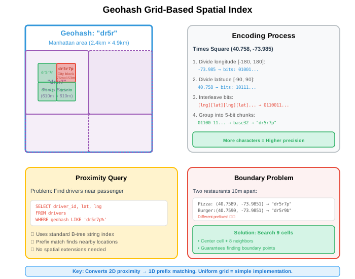
Geohash encodes locations as strings by dividing the world into a uniform grid. Each character adds precision by subdividing the current cell.
Nearby locations share string prefixes. This converts 2D proximity into 1D prefix matching, which B-tree indexes handle efficiently.
Encoding process:
Start with the entire world. Divide it in half by longitude, then latitude, alternating. Each division adds one bit (0 or 1). Group bits into 5-bit chunks and encode as base32 characters.
Times Square (40.758, -73.985):
- Longitude -73.985 in range [-180, 180]: bits 01001...
- Latitude 40.758 in range [-90, 90]: bits 10111...
- Interleave: 0110011... → base32: "dr5ru7"
Precision levels:
"dr5r"   → 39km × 19.5km
"dr5ru"  → 4.9km × 4.9km
"dr5ru7" → 1.2km × 609m
Database queries:
Ride-sharing apps store driver locations as geohash strings. Finding drivers near a passenger requires a simple prefix match:
SELECT driver_id, lat, lng
FROM drivers
WHERE geohash LIKE 'dr5ru7%'
  AND status = 'available'
The database uses its standard string index. No spatial extensions needed.
Choosing Between Approaches
Data distribution determines which method works better.
QuadTrees adapt to density. They excel when data clusters unevenly. Food delivery in NYC has dense Manhattan (10,000 restaurants/km²) and sparse Staten Island (50 restaurants/km²). QuadTree cells split only where needed, keeping memory usage low.
Geohash provides uniform coverage. It works well for relatively even distributions. Ride-sharing services spread across entire cities. Weather monitoring covers regions uniformly. IoT sensors deploy in regular grids.
Query patterns matter too. Geohash converts spatial queries into string prefix matches, which any database handles with standard indexes. QuadTrees require spatial libraries or custom implementations.
| Factor | QuadTree | Geohash |
|---|---|---|
| Dense clusters | Adapts automatically | Fixed cell overhead |
| Sparse regions | Efficient (large cells) | Wastes empty cells |
| Query complexity | Tree traversal O(log n) | Index range scan O(log n + k) |
| Database support | Needs spatial extension | Standard string index |
| Updates | Rebalancing required | Direct insert |
| Implementation | Complex | Simple |
Limitations of Basic Approaches
Both methods have weaknesses that matter at scale.
QuadTree challenges: Tree rebalancing costs grow with updates. When thousands of restaurants open and close daily, rebalancing operations compete with queries. The tree structure also requires custom spatial libraries or database extensions. Not every database supports QuadTree indexes natively.
Geohash challenges: Rectangular cells create edge cases. Locations near cell boundaries fall into different geohashes despite being close together. A query must inspect enough neighboring cells for its radius and latitude, then apply an exact distance filter. Nine cells (center plus 8 neighbors) suffice only when the selected cells are large enough relative to the radius. More importantly, rectangular grids distort at high latitudes. A geohash cell at the equator covers a different area than one at 60° latitude.
The boundary problem affects both approaches. A search radius intersects multiple cells or tree nodes. Production systems must handle this, adding complexity. Cell shape matters too. Rectangles have 8 neighbors at varying distances. This creates bias in distance-based queries.
Advanced Approaches
Advanced spatial indexing methods address the limitations above.
H3 Hexagonal Indexing solves the edge bias problem. Hexagons have 6 neighbors all at equal distance, unlike rectangles with 8 neighbors at two different distances. This uniformity improves distance-based queries and aggregation. Uber built H3 for global driver-passenger matching. The hexagonal grid remains a grid-based approach but with better geometric properties than rectangular Geohash.
Google S2 reduces Geohash's latitude distortion. S2 projects the sphere onto a cube, then subdivides each face and orders cells using Hilbert curves. Cell areas still vary, but far less systematically than longitude-width cells that shrink toward the poles. The Hilbert ordering preserves useful spatial locality. S2 is fundamentally a hierarchical spherical grid rather than a latitude/longitude rectangle scheme.
Hilbert Curves improve how grids map 2D space to 1D. Simple geohash interleaving creates locality problems at cell boundaries. Hilbert curves map nearby 2D points to nearby 1D positions more consistently. This reduces the boundary problem, though not entirely. Google Bigtable applies Hilbert curves to row key design for better range scan performance.
These advanced methods build on the same principles: either adaptive tree structures or uniform grids. H3 and S2 refine grid-based indexing with better geometry. QuadTrees remain effective for dynamically clustered data.
Spatial indexing transforms O(n) linear scans into O(log n) tree traversals or near-constant grid lookups (index range scans over a cell prefix). Choose QuadTrees when data clusters unevenly. Choose Geohash when simplicity and standard database support matter. Consider H3 or S2 for global-scale applications requiring geometric consistency.
The following articles explore each approach in depth. Geohash shows the encoding algorithm and boundary handling techniques. QuadTrees covers tree construction, balancing strategies, and range queries. H3 Hexagonal Indexing, Space-Filling Curves, and Google S2 examine advanced methods with production examples and trade-off analysis.