Data Structures Behind Databases
Every database keeps its records in files and must answer two questions about each record: where to write it, and how to find it again. The storage engine is the part of the database that answers both questions, and its underlying data structure decides which operations are cheap. One structure accepts a write with a single sequential append, but it cannot list a range of keys. Another answers range queries directly, but it rewrites a whole page for every small change. PostgreSQL stores its indexes in one kind of structure while Cassandra stores its data in another, so the two handle a heavy write load differently.
Sequential and Random Writes
Storage hardware writes data much faster in sequence than at scattered positions. Each sequential write lands right after the previous one in the file. In contrast, each random write lands at an unrelated position.
On a hard disk drive (HDD), a write must wait for the read/write head to move to the right track and for the platter to turn under it. Consider a disk where this wait takes roughly 10 ms. That disk completes about 1,000 ÷ 10 = 100 random writes per second, which is only 400 KB/s if each write is 4 KB. During sequential writing, the head stays in place and the data streams onto the track at a rate on the order of 100 MB/s on the same disk.
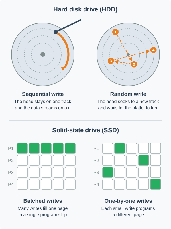

Solid-state drives (SSDs) have no moving parts, so the performance gap is smaller. The gap does not disappear. The smallest unit of writing in flash memory is a flash page. Flash memory cannot overwrite a flash page in place. Instead, the drive writes new data into erased flash pages and erases a whole block of many flash pages at a time. Scattered small writes leave live and stale flash pages mixed inside each block. Before the drive can erase such a block, it must copy the live flash pages elsewhere, creating extra internal writes. Sequential writes fill and free whole blocks together, so the drive copies far less data.
Storage engines that turn their writes into sequential appends therefore get more throughput from the same disk. The log, the hash index, and the LSM tree in this section all build on this idea, whereas the B-tree takes the other side of the trade-off.
An Append-Only Log
A minimal storage engine is a single file that only grows. This file is an append-only log. Each write appends a line with the key and the value to the end of the file. Each update appends a new line for the same key, so the newest line wins. Each delete appends a tombstone. The tombstone is a record that marks the key as deleted.
user:1,Alice
user:2,Bob
user:3,Cara
user:1,Alice B
user:3,DELETED
Because every write is a sequential append, writes are as fast as the disk allows. In contrast, reads are slow. To find the value of user:1, the engine must read the whole file because a newer line for the key could appear anywhere after an older one. Each read therefore takes time in proportion to the size of the log; with 10 million records, every read checks 10 million records.
The widget runs eight writes against an append-only log. Press "Step" until all eight writes are in the log, then press "Get user:1". In "Scan the log" mode, the read checks every record and keeps the last match for the key.
Hash Index
A hash index removes the full-file scan. The engine keeps an in-memory hash map from each key to the byte offset of its newest record. The offset is its position in bytes from the start of the file. On a write, the engine appends the record to the file and updates its offset in the map. On a read, the engine looks up the offset in memory, seeks to that position in the file, and reads a single record.
Switch the widget to "Hash index" and press "Get user:1" again. The read now goes straight to the newest record and reads one record instead of eight. Deleting a key removes it from the map, so "Get user:3" finishes without reading the file at all.
Bitcask, the default storage engine in the Riak database, works this way. Its in-memory table, called the keydir, maps every key to the file, position, and size of its newest value, so a read needs at most one disk seek (Bitcask paper).
The code below builds this store in Python: an append-only log file with an in-memory index of byte offsets. Run it, then change the calls at the bottom to set, update, and delete other keys.
Simple File-Based Key-Value Store
Compaction
The log still keeps every old version of a record on disk. After the eight writes in the widget, the log holds 8 records but only 3 live keys, leaving most of the file as wasted space. Compaction reclaims this space by rewriting the log with only the newest record of each live key while dropping stale versions and deleted keys. Press "Compact" to see the log shrink. Real engines split the log into segments. Each segment is a file of a fixed maximum size. They write new records to the active segment and compact the older, frozen segments in the background, so compaction runs without stopping new writes.
Limits of the Hash Index
The hash index fixes the read cost. The cost is two new limits.
First, every key must fit in memory because the map holds one entry per key along with its offset. Consider 100 million keys at about 50 bytes per entry, including the key, the offset, and the hash map overhead. That map requires about 100,000,000 × 50 = 5 GB of RAM, and it grows with every new key.
Second, a hash index cannot answer a range query. The hash function scatters neighboring keys across unrelated buckets, leaving the map with no notion of order. So a query for "all users from user:1000 to user:1999" must look up each of the 1,000 possible keys one at a time, or check every key in the map.
Keeping the keys sorted solves both limits. In sorted order, a range forms one contiguous stretch of data, so a range query reads sequentially from the first key to the last. The index can also be sparse, storing one entry per block of keys instead of one per key, because any key between two index entries must sit in the block between them.
Two Ways to Keep Keys Sorted
Databases keep keys sorted on disk in one of two ways, which differ in how they handle writes.
A B-tree stores keys in fixed-size pages arranged as a shallow tree. Each write finds the page that holds its key and rewrites that page in place on disk. Each read follows a single path from the root to a leaf. Writes land wherever their target keys live, so they are random writes. PostgreSQL and MySQL's InnoDB store their indexes this way (PostgreSQL docs, MySQL docs).
A log-structured merge tree (LSM tree) keeps the append-only design. It collects incoming writes in a sorted in-memory buffer. When the buffer fills, the engine flushes it to disk as a new sorted file in one sequential write. Each immutable file is a Sorted String Table (SSTable). Over time, a background process merges them into larger files. RocksDB, LevelDB, and Cassandra store data this way (RocksDB wiki, Cassandra docs).
The LSM tree pays for its sequential writes at read time. Because a key can sit in the memory buffer or in any of several on-disk files, a read may need to check multiple places. The background merges also rewrite the same data several times over its lifetime.
Choosing a Structure
The three structures trade write cost, read cost, and memory usage against each other.
| Structure | How a write reaches disk | Point read | Range query | Memory needed |
|---|---|---|---|---|
| Hash index on a log | Sequential append | One record read | Not supported | Every key |
| B-tree | Page rewritten in place (random) | One path down the tree | Scan of adjacent leaf pages | Upper tree pages, as a cache |
| LSM tree | Sorted buffer flushed as a new file (sequential) | May check several files | Merge across several sorted files | Write buffer and small per-file indexes |
Hash indexes on a log suit a key space that fits in memory and needs only exact-key lookups. B-trees suit workloads with heavy reads and range queries, such as most transactional databases. LSM trees suit write-heavy workloads like event logs, metrics, and messaging, where sequential writes absorb a high write rate.
Key idea. An append-only log turns every write into a sequential append, while an in-memory hash index of key offsets lets a read fetch a single record. The cost is that a hash index must hold every key in memory and cannot answer range queries. B-trees and LSM trees keep keys sorted to remove both limits: a B-tree rewrites fixed-size pages in place, whereas an LSM tree writes new sorted files sequentially and merges them in the background.
The next lessons cover each sorted structure in detail. B-tree explains how pages split and why the tree stays three or four levels deep. SSTable covers the sorted file format, its sparse index, and how two files merge. LSM tree walks through the full write path, the read path, and compaction.
Further Reading
- Bitcask: A Log-Structured Hash Table for Fast Key/Value Data — Sheehy and Smith, Basho: the append-only log with an in-memory hash index, and its merge process.
- The Log-Structured Merge-Tree (LSM-Tree) — O'Neil, Cheng, Gawlick, and O'Neil, Acta Informatica, 1996: the paper that introduced the LSM tree.
- RocksDB Overview — RocksDB wiki: the architecture of a widely used LSM storage engine.
- B-Tree Indexes — PostgreSQL docs: the B-tree implementation in PostgreSQL.